Analyzing Markets at Scale — A Crawling Blueprint

Posted on 2017-10-29

Crawling and scraping sounds like this one-time flaky quirky work. But what kind of products or companies need this for their core offering?

Price tracking and comparative websites like newegg.
Search engine optimization (SEO) and app store optimization (ASO) products.
Market analysis and optimization companies, like SimilarWeb and AppAnnie.

Building for this kind of scale needs reliable and scalable crawling and data architectures for its core offering. These requirements reveal the following, sometimes conflicting, challenges.

Information retrieval. The source of our data are websites, but not limited to that. It can also be PDFs, spreadsheets, and APIs. These sources can vary in the degree of friendliness towards us.
Natural language processing. Data normalization, and the semantic web. Wide fields of research, but we still have to do a bit of each when presented with painfully unstructured pieces of data.
Networking. Traffic routes and counter-protection. Crawling and scraping involves taking in a big and complete amount of data in a short amount of time, sometimes targeting resources that aren’t built for it or (without us taking a side in the legal aspects of it) not interested in it happening, for reasons such as terms of service and more.
Big data pipelines, aggregation and analytics. With almost any crawling infrastructure, we’re bound to pile an ever-increasing, large, amount of data with every job and every time unit (hours, days, weeks).
Speed layer and search. Almost all crawling solutions need some kind of speed layer. One that can provide answers for a subset of the questions in real-time, rather answering all questions after a long while.
Agility. Our target data sources change (read: websites), our auxiliary data sources change (read: exchange rates), and our requirements change (read: features). This kind of multiplier of change requires an agile turn-around operation to compensate throughout crawling, data pipeline, and search (read: rebuild, rerun, reindex).

And a ton more. You’d be surprised at how many products you use every day that build on a core set of data that’s they source from crawling, and that fact is swept to the back of the stage, because crawling, data cleansing, and flakyness is not cool and no longer as marketable as it was in the past.

General Architecture

We’re going to deep dive from a general architecture for crawling and data processing that deals with a crawler, a batch layer and a query layer like this:

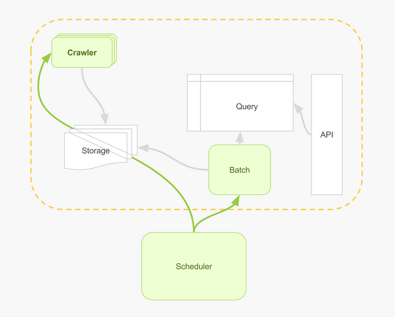
Into something more prescriptive that you can actually use, naming the components and tools that I use in production, like this:

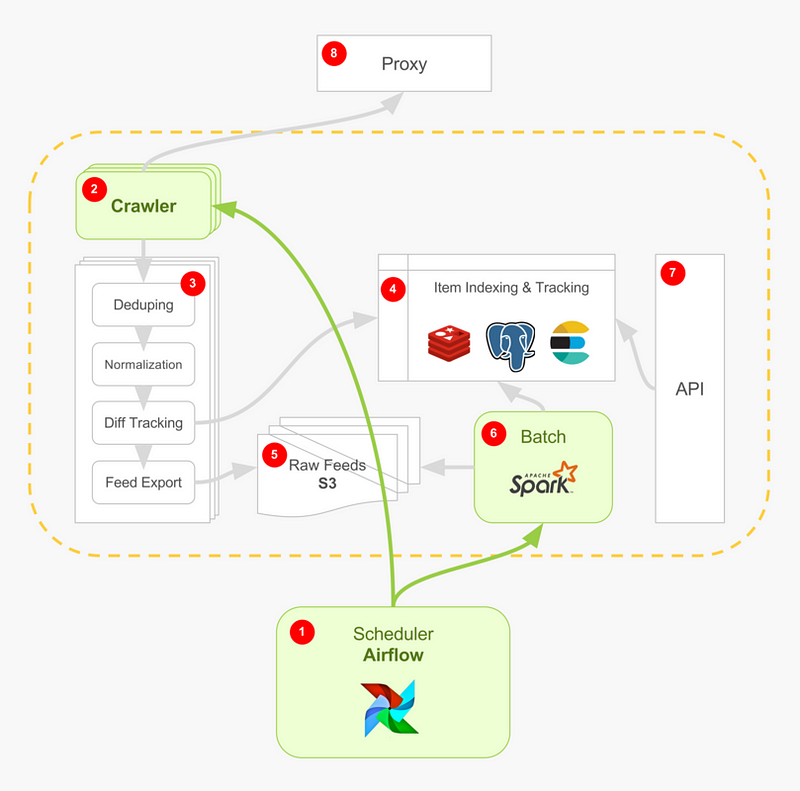
Here’s how the flow works.

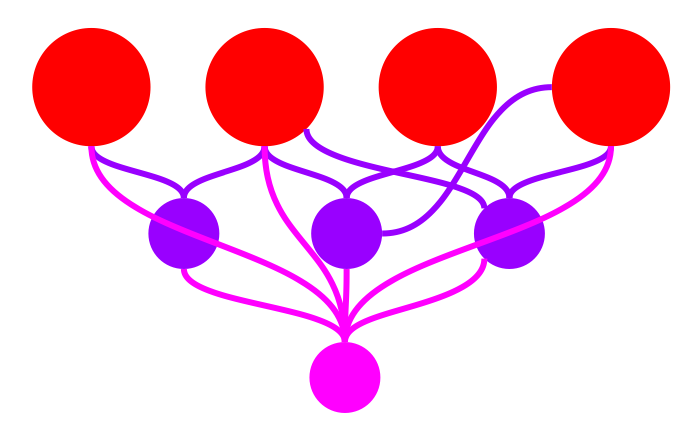
Scheduler (Airflow) fires off a new crawl job, specifying the current time unit for this job. It may fire off several of these jobs for redundancy, as crawling is flaky; accepting that we’ll have duplicate data from the get-go. We’ll also start auxiliary crawls to enrich our data, such as fetching exchange rates from dedicated brokers. The scheduler is also responsible to coordinate and converge the jobs it started as a graph.
For each target, our crawler goes out through our proxy (8), fuzzing out a request IP, user agent, data center and so on, and handing back a raw HTML content (for when the target source is a website).
Each candidate web page goes through an internal crawler pipeline which does a subset of the data manipulation needed: deduping, normalization, item tracking and item export.
At the tracking stage, we drive items towards a cache to make sure to drop duplicates, and onto a search engine, available for query in real-time.
Items piled up in data feeds on S3 as the job progresses. When done, we’ll have a bunch of JSON files for a main crawl and its redundancy crawls as well as any auxiliary crawl that we fired off.
Finally, Airflow (1) starts a data flow job, using sensors to detect when data is available.
We load job data results onto the indexing & tracking component (4) for a most-up-to-date view of the world, using a relational database such as Postgres, to provide an OLAP style querying solution.

Let’s have a deep dive into every component, and put some more content behind what this architecture means practically.

Crawler

Scrapy makes an agile and flexible crawling and scraping platform. It provides the quickest turn around from an experiment to a production project. Still, it’s not a broad-crawl platform like Nutch is, and the mindset is different.

In the Scrapy mindset you crawl and scrape, extract content in one go, patch up any difficulties you might have while crawling, including any logic for coalescing or cleansing data types and navigating the target site more effectively; for example, normalizing product prices or making sure Javascript fragments get rendered before scraping.

In the Nutch mindset, you download a chunk of the internet. You then perform a big-data pass on the raw results to form structured data. There’s flexibility in crawl time, should you want to be more agile, but it’s done through configuration and plugin setup rather than code.

If you’re new to Scrapy, I recommend looking at a sample crawler and a more realistic crawler to get the gist of it; it’s self explanatory because Scrapy does the heavy lifting for you. What’s less obvious to newcomers is the extensibility points and plugins Scrapy comes with and how does a fully rigged solution look like, so let’s take a look at some of the more popular components around it.

Scrapy revolves around simple concepts.

Spider. What ever is doing the crawl, maintains the crawl frontier, lifecycle, moves pages through your code, and then onto the pipeline.
Pipeline. All discovered items go through the pipeline; which can be an empty one, or one that flushes items to files by format — CSV, JSON or what have you.
Middleware. Pieces of code that wake up during the different stages in the spider’s lifecycle. One example is a middleware that will randomly swap user agents for each external request.
Configuration. On first glance sounds pretty static and trivial, but here it behaves much like feature flags for your crawler since your configuration file is code. Some ideas are to activate or disable your pieces of code per variant of a crawl, swap a piece of infrastructure (anonymising proxy), or perform staging and test runs if you’d like — all by remotely/locally specifying flags per run.

Delta Crawls

A delta crawl is a crawl process that will output new or changed items, since the last crawl which makes a smaller incremental addition to our data set. To do that, Scrapy has to store some kind of state.

With pgpipeline we use a database for book keeping; here Postgres but most relational databases Python supports work. While pgpipeline does more than modeling delta crawls (more on that later), it supports being able to store new/modified items to your database automatically.
With deltafetch the book keeping is at the page level; ignoring pages that we saw in previous crawls. A less flexible solution than pgpipeline but still works for modeling delta crawls on a file system, which everybody has.

Throttling/Anti-crawler Bypass

If you’re trying to bypass someone’s protection mechanisms or terms of service — that can be illegal to varying levels of degrees.

I’ll assume we have some kind of funny situation where we’re crawling against your own company, let’s say for security or compliance, and, say, that this other team that’s responsible for the target website cannot lift their protection mechanisms for you or don’t have the time to build something that conditionally does it for you.

There, we cleared our conscious.

For bypassing crawler-circumventing mechanisms, one sure way is to use (without promoting any of those) either of the following plugins, to make sure requests fan-out through different IPs.

crawlera — anonymising proxy.
proxymesh — anonymising proxy.
tor — anonymising proxy, using the Onion Network.
open proxies, and probably more to make sure the crawler agent’s IP gets changed every now and then. From experience that’s the most effective way to thwart most protection schemes.
User agent faking and swapping is also useful to avoid blacklisted user agents.

These reverse proxies can be very slow, as some providers can take minutes(!) of response times when swapping IPs and that some of the providers (e.g. ProxyMesh) were’nt built for crawling purposes with all the related implications (legal, performance, etc.).

Alternate Rendering

To render pages with active Javascript, we can use Splash. That said headless chrome API was out earlier this year, which sparked a ton of out-of-band rendering libraries, a gold mine for crawlers.

When we do Javascript renders, our crawls become slow because there’s a browser of some sort that needs to go out and fetch data from an API and then complete a page’s render. Depending on feasibility, it’s preferrable to do auxiliary crawls that target the Javascript API individually and merge this data as part of the merge job; leaving us in a simple and fast HTML render domain.

Crawl Persistence

Scrapy has a built-in ability to cache crawl sessions, and resume sessions. If enabled, a .scrapy folder will appear, and in it a pickled storage of the last crawl activity, which it will use for next crawls as a cache.

Regardless, we can use the following to augment or replace this capability.

pagestorage stores requests and responses.
dotpersistence will sync the Scrapy .scrapy folder to S3.

Data Normlization

Other than using any Python library out the for data normalization (and there’s a lot), we can use Scrapy plugins that streamline that into your pipeline. Here’s a couple useful ones.

magicfields allows us to add standard fields to a scraped item (timestamp, etc.).
querycleaner helps cleaning a noisy item URL, so that two identical items under slightly different URLs with referrers and arbitrary query params are semantically the same.

Notifications

Scrapy do notifications via different channels out of the box (that includes SMTP). A job started, ended, failed and what were the statistics is useful to keep from one crawl to another. We can also find 3rd party integrations such as Mailgun that is smooth to use with the simplicity of an API key and a couple configuration values.

Storage and Indexing

Scrapy has plugins for dynamodb, mongodb, Elastic Search which is useful, and pgpipeline for automatic persistence to Postgresql (and probably more).

We can also dump scraped items to SQS and from then get a worker to take items off the queue and persist as you’d prefer.

Crawling and CI/CD

Scrapy runs as its own process by default. But there are other ways, perhaps more creative, to repackage and run it.

As an embedded Python codebase. We can embed your crawler in an existing program or service; for example, we can crawl on-demand triggered by some agent making a request, and provide crawl results to the requesting agent when done.
We can build a worker farm, where each worker runs a spider of its own. One implementation can be Jenkins and Jenkins workers, or Docker and ECS (my preferred way).

As soon as you’re able to dockerize your crawler, a compute unit that can run Docker and a place to dump results is all you need. I’ve ran the same crawlers on a home array of Raspberry Pi’s, on Docker Cloud, on ScrapingHub and on ECS and it was perfectly transparent.

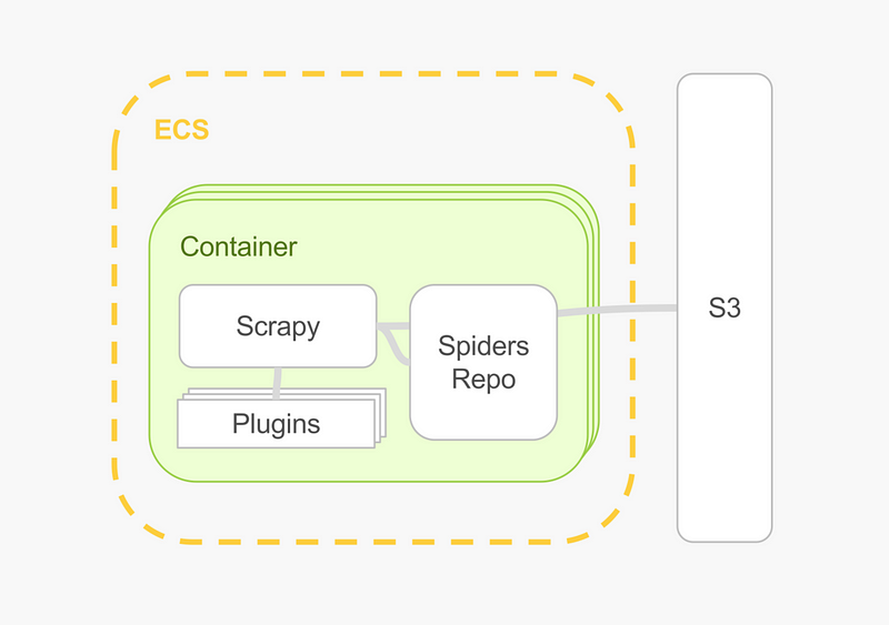
To be most effective, bake a container with everything in it; Python, Scrapy, as many plugins as you like, and your spiders code and configuration. The moment the container is up, it should start crawling.

Running specifically on AWS can be cheap and powerful (more on processing data later), and flexible for data integrations. Use ECS (a small instance will do, as this is an I/O bound workload) and dump data directly on S3.

Proxy

Go out to the world to fetch bytes through a proxy. Using an anonymising network — that’s already happening. Using a proxy on top of that, or without that can be beneficial.

Caching and micro-caching. Even with Scrapy’s local file-caching feature, an HTTP caching proxy will give us better and more familiar levels of control for caching, and allow horizontal scaling when several crawlers are involved.
Blocking sites and re-routing at the proxy level. Malfunctioning sites, network components will require our intervention. With a proxy sitting between a crawler and the world, we can remote flip a switch for a strategy to amend such problems.
Rerouting through other proxies towards other data centers. We might decide to flow part of the traffic through an anonymising network and some of it out directly, or through a bunch of anonymising networks.

In any case, we also get visibility for free from most proxy products: how many requests succeeded, failed, in-flight, latency, size of payloads and more.

Pipeline

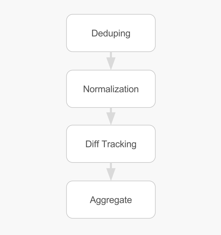
The Scrapy pipeline is the place where we do deduping, normalization, diff tracking, exporting and more. It’s the place where extracted data flows through.

Almost everything mentioned here can be done on raw data in batch much later. Which steps do we do in Scrapy’s pipeline and which steps do we save for the, later, offline run?

First, do we want to have a data pass after crawling has finished? if we’re still small, we’d probably want to keep everything together and skip that amount of extra work; and that’s fine, Scrapy will let us do that. In that case everything mentioned can be done in the pipeline, during the crawl.

If we do have an offline step already planned or set up, then steps like deduping, normalization diff tracking will be perfect there. We won’t have to split that kind of logic across two process and perhaps codebases. When we’re looking at all of the data we’re also smarter and have more context to do these operations; and we can also move faster and trial our ideas on that data, without invoking any lengthy and flaky recrawl process (because they always are flaky).

That said, there are a few tasks we do want to perform during the crawl in Scrapy’s pipeline. These are tasks that are time-sensitive; one example would be performing IP to location, calls to 3rd party APIs or data conversions such as exchange rates.

Feeds

When we crawl a website, we ultimately want to end up with a list of items. With Scrapy we can have that list automatically serialized and exported through the feeds mechanism; it can be JSON, CSV, or what have you, through plugins that set themselves up at the end of your pipeline.

When picking a format, JSON is a good bet, although it is verbose. For ad-hoc crawls I tend to use CSV, which fits well with the rest of the data wrangling toolset existing in Python, like pandas. For production I always use JSON. For JSON — keep your objects flat, don’t nest.

Either case, when we’re running multiple crawls that should converge on the same entity, such as a baseline crawl and multiple auxiliary enrichment crawls, make sure there’s already an ID, or a strong strategy to join the data from the auxiliary crawls onto the baseline crawl; we don’t want to look for how to massage our data fields to join on after we’ve realized it can’t be joined, risking dumping the data and recrawling everything.

One other thing — always output more than needed. It’s best to include a field when unsure rather than optimize it out of the data feed.

Item Indexing and Tracking

Building a crawling solution, we’ll require a way to provide search. Search makes data accessible for slicing and dicing, and immediately accessible in terms of real-timeness. It’s a quick win to bypass all other heavy work we’re going to do in our batch layer; this is our speedy data solution for random access use cases.

When we use Elastic Search to index our data, we get a pretty good API for free, and plenty of UI interfaces to use for our backoffice. Not to mention a bullet proof search product that scales with our data.

Inflight item indexing is another technique we should use. We want to prevent duplicate work while running a crawl, which means we must identify when an item was already crawled and effectively dedupe it. For this, we’ll need an extra state store. Redis makes a perfect match both in speed and features. We can store actual items via key/value, or use a statistical counter like HLL which Redis also has.

Lastly, we push aggregated data onto Postgres for more traditional OLAP-like querying.

Batch Layer

When all crawls finish, we need to do some data crunching. Matching options for different scale are pandas , petl, pytables, Apache Spark.

The basic idea is that given a way to load crawl result feeds from anywhere, process using split-apply-combine, map/reduce, or SQL-like grouping and aggregation, and, dump back into anywhere (databases, files). We want the tooling we use to have a great coverage of inputs and outputs; from/to S3, databases or others, and great aggregation and data join abstractions including flexible or programmable logic for prefilling and merging values when joining multiple datasources (more on that later).

Scheduling

We schedule two job types regularily: crawling jobs and data processing jobs. Ideally one is upstream to the other but not necessarily so. Even if a crawling job generates data, and a data processing job kicks to process it, and we know that is a linear action-reaction dependency, we can still run data processing regardless, retroactively, as time moves forward and we discover new facts about our data. This includes fixing inconsistencies, taking out stale items, or as a practical example, updating a comment count on items that we’ve discovered earlier.

To schedule these kind of jobs I recommend Airflow and Jenkins. To make a choice between the two, you’re welcome to read my earlier article about Airflow where I pour some context into the “why Airflow” question.

Sticking to Python, we can actually embed Scrapy with our spiders, and a PySpark job into an Airflow DAG.

Airflow, unlike Jenkins, will lets us generate crawls dynamically as we see fit. One example is that we can have the same crawl needed to run for different markets, and the markets change with time. Within an Airflow DAG, we generate the current crawl tree based on the current spread of markets; the crawl codebase is always the same but every run tweaks a few settings that turns on or off a bunch of crawl paths.

Another nice feature from Airflow over Jenkins is that it has backfilling as a first-class concept. When dealing with crawl data, there’s a ton of mistakes or errornous crawls that we know we want to rerun even shortly after a crawl had started. A great strategy to adopt is one that redoes previous crawls as a safety guard every now and then; Airflow’s backfilling takes away all of the back of envelope calculations to figure out which dates to rerun.

Data Handling

Let’s imagine we only dealt with files. Each crawl job outputs data feeds with items that it discovered. Other enrichment jobs do the same, dealing with the same structure of data. All jobs have a common way to determine an item_id or to synthesize it from the rest of an item's properties, i.e., as item_url+item_SKU.

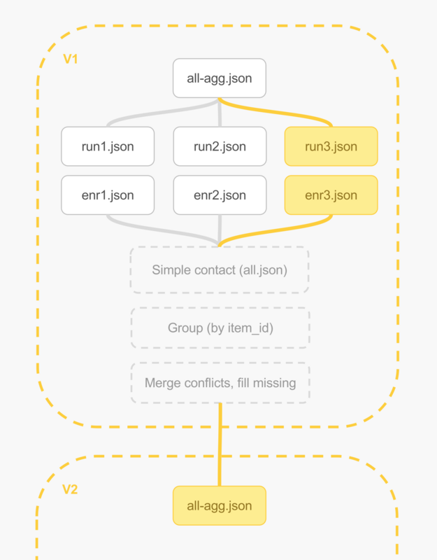
Crawl by fielding N jobs, we can partition the data by splitting crawling for different sites or different sections of a site, plus jobs for enriching our base crawl data. All jobs output the same item structure, and blanks where missing.
Take all new and old data files aggN.json, enrN.json and concatenate, for any number of files that there are, it doesn't really matter. At this stage we know we have duplicates, older runs and new run, and possibly we have duplicates in our own current data run - that's all OK.
We now group all data to discover unique items, we merge conflicts when items are the same. One strategy is to take the newer item over an older one when properties conflict, or take a richer property from either copy, and fill blank properties from newest run.
We’ve now created a new world view all-agg.json based on all known runs. This view is aggregated and clean, so we can load it onto a relational database for querying, or onto a search engine.

An alternative to step (2) would be to take the latest known worldview, all-aggN.json and concatenate with the new run runN+1.json, resulting in all-aggN+1.json, acknowledging that we're doing a running-average like operation.

Trying to reduce this flow to mechanical operations, here’s how it should look like after a few runs.

# 'run-N' is a base crawl
# 'e' is an enrichment crawl
# 'wv' is a world view

run-1, e1  ->   wv1 ( = run-1)
run-2, e2  ->   wv2   (= agg(run-2, e2, wv1)
run-3, e3  ->   wv3   (= agg(run-3, e3, wv2))
run-4, e4  ->   wv4   (= agg(run-4, e4, wv3))
...

Using a Database vs Files

Illustrating this process with simple files is both more intuitive and more scalable for when databases can’t hold the dataset we care about. However, when we don’t aim for high scale from the start, we can definitely use a database instead. The big advantage is that we can iterate much faster, have less moving parts and probably pay less if we don’t really have a full big data infrastructure online processing these files.

(a) Files only

Data is in a distributed file store and processed with a big data pipeline.

Principles

Handle files, since beginning of time, for each revolution of the data model. This lends itself well to a big data — data warehouse settings. Secondly, we always have the raw collected data should we want to go back.
Cut chunks of the data flow to atomic processing tasks: deduping, merging and so on.
Aggregation using an aggregation model ad-hoc (map/reduce, SAC, SQL over files).
Load to one or more data store(s), with an infrastructure and query-optimized data model.

Pros

Always have raw collected data. With it, we can change the direction of our product in a stateless way, without rummaging through our existing processed datasets trying to figure out what’s good and what’s not. Simply rebuild, on the expense of compute power.
Can apply different kinds of fire-power when needed. We can do data processing by employing some batch infrastructure (spark), and data querying and analysis by employing different storage engines or multiple storage engines optimized for retrieval.
Better parallelism. We can break creation of data to several processes (e.g. each scraper taking a vertical) and merge files later; as well as perform data enrichment before loading it to a store.
Breakable. We can break this proble onto teams or people, assigning tasks to specialty without each stepping on another’s toes.

Cons

Elaborate to ship data. We need a reliable data shipping process and something to keep track of it.
Slower progression. Since we’ve broken up our pipeline we have multiple moving parts and relatively slow communication between those.

(b) Files + Database: Hybrid

Using our database as a state book keeper.

Principles

Files only exist for the current job; which we get anyway from our crawling infrastructure.
Via ETL process, target reach new record in aggregated files against latest world-view in our database to perform merge.
Result is a new world view, in our database
Rebuilding the world-view is re-applying this process against all files and an empty database serially

Pros

Simpler. Same process as (a), only that now we use a “scratch book” for book keeping our world view; which means less moving parts (read: files) to aggregate against and coordinate data shipping.
We keep scalability for crawling, in case we want to break our crawl data generation to several sub-crawls.

Cons

Risks of state being corrupted and/or propagating error through the main database.
Merging data against our main database will create a stop-the-world like churn every cycle.
Scaling up means scaling a database, until we have to dump it.

(c) Database

Treating our database as an abstract file store.

While crawling, each item is directly inserted into our database (minus trivial deduping) into a current-run “raw” table.
A batch SQL job loads “raw” table or multiple “raw” tables and aggregates into a new table, which stands for our current worldview.
When our “raw” table(s) represent all data from all previous runs — conceptually similar to (a), when our “raw” table is just the last run against a main table — conceptually similar to (b).

Pros

No need to deal with files: storage and shipping. Data is shipped via a persistent connection to our database.
Saving all data in “raw” form, without processing and indexing, helps with database performance.

Cons

Single point of failure at worst, dealing with high-availability downtime at best.
Waste is generated by constantly pushing raw data and trimming it down by aggregation.

(d) Database Only: Item Loader

Each record discovered is immediately trialed against a database.
Datbase helps with deduping.
Aggregation is made against the last clean and aggregated state in database.
Enrichment or cross-item data processes is done with independent tables and linked via joins.

Pros

Simplest. No file handling, data is shipped easily.
No moving parts, an all-in-one, rapid solution.

Cons

Risks of corrupting data propagating errors.
High complexity when we want to break data generation (parallel crawls) into multiple stages (each stage competes for database access and data races).
Escalates into being a major bottleneck fairly quickly.

Aggregating Data: Starting Points

We’ll take a look at the following dataset, crawled from an imaginary fashion website. This dataset includes two runs (a, b), and part of the items are discovered in both runs, featuring price and rating updates.

id,job_id,name,desc,price,reviews,rating,featured
"1",a,"black t-shirt","a pitch black t-shirt for every occasion",90.99,303,4.5,
"1",b,"black t-shirt","a pitch black t-shirt for every occasion",95.99,303,4.5
"1",a,"black t-shirt","a pitch black t-shirt for every occasion",90.99,308,4.5,1
"2",a,"blue dress","a plain blue dress",110.00,2,2.0,0
"2",a,"blue dress","a plain blue dress",110.00,2,2.0,1
"2",a,"blue dress","a plain blue dress",110.00,2,2.0,1
"2",b,"blue dress","a plain blue dress",110.00,2,2.0,1

We need to take this data set, and aggregate it. Here are a few notes about this aggregation.

First we want to build a record set that forms the baseline of all our items, an “epoch” of our worldview. We can take these from our first job (job id=a).
Next, perform diff tracking by identifying items that changed through all successive jobs (job id=b, etc.), and only for those items add records that describe an updated item. Items that are completely identical between runs are dropped.
Diff tracking logic can change from application to application. For this instance, we say that an item can still be the same if it has a different description (we don’t care we just take the first one we see), but we observe a change if its price changed.

Here’s how it looks like using pandas, a data science oriented toolkit:

And petl, a slightly more ETL oriented toolkit:

For this last example, I’ve used a different dataset that I pulled from production. Avoiding the annoyance of including this data set here, the principles are the same minus the field names.

Lastly, if you want to strictly deal with putting items on a database, I’ve encoded a flexible set of conflict resolution that you can use for diff tracking logic into pgpipeline, a Scrapy plugin that hooks directly into your spider pipeline and with it, you can describe how to add, index, merge and track items.

Summary

The hardest task for building this kind of product is making the right choices for each component and building something that can start small, iterate fast, and scale up with little to no effort.

The architecture and technical choices presented here started small and scaled up without requiring re-engineering. It’s delivering a market analysis product that works at scale, covering stores with tens of thousands of products.

There’s a more detail to share, but I’ve been painfully careful to not have a narrow view and describe this one specific product but a family of products fitting this domain, so that you can observe the pattern, context, and decisions that are needed to succeed.